Blog
How to Enhance Forecasts of the Scottish Economy with New Hire Wages and Machine Learning
1. The SFC’s Core Methodology: A Structural Foundation
The Scottish Fiscal Commission (SFC), an independent institution responsible for economic and fiscal forecasting to accompany the Scottish Government’s Budget cycle, published a technical report on May 2021 describing their operational motivation, methodology and underlying assumptions. The report establishes the process behind the forecasting of trend GDP – defined as the maximum amount of goods and services the economy can sustainably produce – and presents a decomposition mechanism that breaks this task into several, smaller forecasting and/or calibration exercises: namely, a list of endogenous variables comprising the unemployment rate gap, private-sector real hourly wage and household consumption.
In this blog post, I want to focus on the stochastic process – an error correction model - governing private-sector real hourly wages and illustrate how two key changes can help improve the accuracy of the forecasts. First, following Pissarides (2010) I propose the distinction between new hire and incumbent private sector real wages. While the distinction made in the report between public and private sector real wages speaks to an important structural characteristic of the economy, wages for new hires are considerably more procyclical than average wages. Hence, the underlying assumption that new hires represent rigid labour costs is a limitation for the short-term component of the ECM (Schaefer and Singleton, 2017). Second, I illustrate how modern forecasting methods leveraging machine learning can outperform traditional econometric models – e.g. ARIMA – when working with short panels, which are prevalent in macroeconomic data. I illustrate the quantitative impact of each of these changes separately, using simulated data in Python, using tensorflow, numpy, pandas and sklearn.
2. Why New Hire Wages Matter: Solving the Unemployment Volatility Puzzle
Traditional models use average wages, which smooth wage cyclicality due to stickiness in ongoing employment contracts and composition effects. Integrating new hire wages into forecasting models offers a more accurate gauge of labor market dynamics than average wages, as new hire wages exhibit significantly higher procyclicality - declining by 2.2% for every 1 percentage point rise in unemployment, compared to just 0.67% for job stayers (Figueiredo, 2021). This disparity arises because new hires (particularly job switchers) face fewer “lock-in” effects from past wage commitments, allowing wages to adjust rapidly to current economic conditions. Composition effects - such as cyclical upgrades in job-match quality during expansions - further amplify this flexibility. For instance, during downturns, firms hire workers whose skills are less mismatched, temporarily suppressing new hire wages without altering underlying wage structures. By capturing real-time marginal labor costs, new hire wages provide a clearer signal of economic turning points than lagging average wage metrics.
To illustrate the potential benefit of using a different measure of marginal labor costs, I simulate a data set with the key statistical properties from the macro-labor literature that capture the main cyclical wage differences:
import numpy as np
import pandas as pd
import matplotlib.pyplot as plt
from statsmodels.tsa.arima.model import ARIMA
from statsmodels.tsa.statespace.structural import UnobservedComponents
from statsmodels.tsa.filters.hp_filter import hpfilter
from tensorflow.keras.models import Sequential
from tensorflow.keras.layers import LSTM, Dense, Dropout
from tensorflow.keras.regularizers import l2
from sklearn.preprocessing import MinMaxScaler
import pywt

np.random.seed(42)
n = 100  # Small sample size
time = np.arange(n)

productivity_trend = 100 + 0.3*time + 2*np.sin(2*np.pi*time/24)

alpha = -0.08  # Speed of adjustment
beta = 0.80     # Long-run elasticity
gamma = 0.20    # Unemployment gap coefficient

unemployment_gap = 0.5*np.sin(2*np.pi*time/12) + np.random.normal(0, 0.1, n)
wages = np.zeros_like(productivity_trend)
wages_newhires = np.zeros_like(productivity_trend)
wages[0] = beta * productivity_trend[0]  # Start at long-run equilibrium
wages_newhires[0] = beta * productivity_trend[0]

# Enhanced ECM with differentiated rigidity
for t in range(1, n):
    # Regular wages: Stronger error-correction, weaker cyclical response
    wages[t] = wages[t-1] + 0.8*alpha*(wages[t-1] - beta*productivity_trend[t-1]) + 0.5*gamma*unemployment_gap[t]

    # New hire wages: Standard sensitivity
    wages_newhires[t] = wages_newhires[t-1] + 2*alpha*(wages_newhires[t-1] - beta*productivity_trend[t-1]) + 1.5*gamma*unemployment_gap[t]

productivity = productivity_trend + np.random.normal(0, 1, n)
wages += np.random.normal(0, 0.5, n)
wages_newhires += np.random.normal(0, 1, n)
I estimate a single-equation error correction model to forecast productivity using wage data. Critical parameters from simulation setup are informed by SFC parameterization. Cyclicality parameter differences between incumbents and new hires are informed by empirical literature cited above. Cointegration between productivity and wages is structurally guaranteed in the simulation due to the data-generating process being known - non-simulated data should be accompanied by the formal stationarity tests, such as Augmented Dickey-Fuller (ADF).
import statsmodels.api as sm
def ecm_forecast(wage_data, productivity, steps=10):
# Converting inputs to Pandas Series
wage_data = pd.Series(wage_data)
productivity = pd.Series(productivity)
df = pd.DataFrame({
'prod': productivity,
'wage': wage_data,
'prod_lag': productivity.shift(1),
'wage_lag': wage_data.shift(1)
}).dropna()
# Error Correction Term (ECT)
df['ect'] = df['prod_lag'] - 0.8 * df['wage_lag'] # β=0.8 from simulation
# ECM specification: Δprod_t = α + γ*ECT + δ*Δwage_t
X = sm.add_constant(df[['ect', 'wage']])
y = df['prod'] - df['prod_lag'] # Δprod
model = sm.OLS(y, X).fit()
# Dynamic forecasting
forecasts = []
current_prod = df['prod'].iloc[-1]
current_ect = df['ect'].iloc[-1]
current_wage = df['wage'].iloc[-1]
for _ in range(steps):
X_forecast = [1, current_ect, current_wage]
delta_prod = model.predict(X_forecast)[0]
current_prod += delta_prod
forecasts.append(current_prod)
current_ect = current_prod - 0.8 * current_wage
current_wage += np.random.normal(0, 0.5) # Simulate wage evolution
return np.array(forecasts)
regular_forecast = ecm_forecast(wages, productivity)
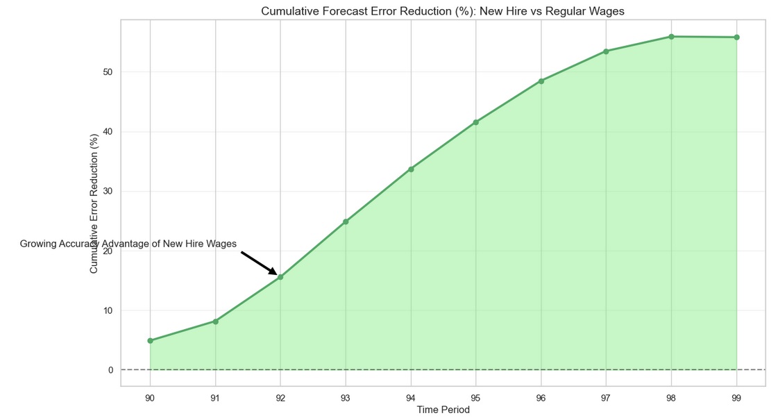
newhire_forecast = ecm_forecast(wages_newhires, productivity)We can then visualize the different covariance of new hire and full sample wages with productivity and, in turn, the value added in model accuracy (measured by cumulative forecast error reduction of using new hire wages in relation to full sample wages):
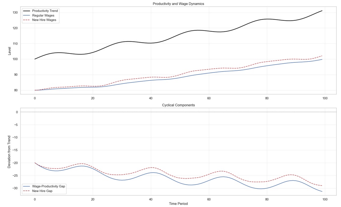
Because new hire wages are more procyclical than regular wages, they are able to better approximate short term cyclical productivity fluctuations than their full sample counterpart. In addition, forecasts using new hire wages provide earlier signals for monetary policy adjustments (Heise, Pearce and Weber, 2025).
Therefore, new hire wages can offer a significant accuracy improvement in GDP trend forecasting by cutting through the noise of wage rigidity. Their real-time responsiveness to productivity and labor dynamics makes them a valuable metric for forward-looking economic analysis. Visualizations of forecast comparisons and cyclical gaps suggest that the argument for their adoption in academic and policy contexts has merit.
It’s important to note that this proposed improvement does not live in the vacuum, and there are other important considerations from recent theoretical and empirical literature that are worth considering, contingent on the policymaker’s trade-off between model accuracy and tractability. Beyond raw cyclicality, forecasting models might also consider skill mismatch heterogeneity and comprehensive labor cost measurement. Wage cyclicality varies across the skill-mismatch spectrum, with mismatched workers showing stronger procyclicality than well-matched counterparts, as shown by Figueiredo, 2021. Additionally, Kudlyak’s user cost of labor framework demonstrates that non-wage expenses (e.g., hiring/training) and match durability elevate adjusted labor cost cyclicality to 4.2–4.8% per 1 percentage point unemployment change - far exceeding conventional estimates (Kudlyak, 2024). Embedding these insights into structural models could shed light into underlying labor market mechanisms relevant to the core macro model and, consequently, refine output gap estimates and potential growth projections, crucial for cyclically adjusted fiscal targets.
3. Machine Learning & ARIMA: A Complementary Toolkit
The ARIMA framework remains foundational in time-series forecasting due to its mathematical rigor and interpretability, particularly for linear trends and seasonal patterns. Its strength lies in modeling stationary data through differencing and leveraging autocorrelation structures via autoregressive (AR) and moving-average (MA) components. However, ARIMA struggles with non-linear dynamics, missing data, and high volatility, often requiring manual parameter tuning. These limitations become acute in complex domains like financial markets, where data exhibits erratic shifts.
LSTM networks surpass ARIMA in capturing non-linear dependencies and long-range temporal patterns through recurrent gates and memory cells. They excel in volatile contexts (e.g., stock prices or epidemic curves) by autonomously learning features without rigid statistical assumptions. For instance, LSTMs reduce forecasting errors by 84–87% in finance compared to ARIMA (Åkesson and Holm, 2024). However, they require larger computational resources and risk overfitting in small samples.
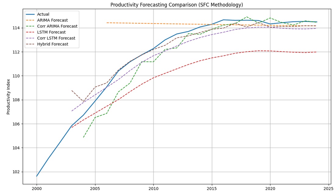
In this section, I use five models to forecast productivity, in line with the SFC’s core trend GDP forecasting methodology:
from statsmodels.tsa.filters.hp_filter import hpfilter

# Computing trend components using HP filter (lambda=1600 for annual data)
def calculate_potential_gdp(df):
    # 1. Trend productivity (HP filter)
    _, prod_trend = hpfilter(df['productivity'], lamb=1600)
    df['prod_trend'] = prod_trend

    # 2. Trend total hours (HP filter)
    _, hours_trend = hpfilter(df['total_hours'], lamb=1600)
    df['hours_trend'] = hours_trend

    # 3. Potential GDP = Trend productivity * Trend hours
    df['potential_gdp'] = df['prod_trend'] * df['hours_trend']

    return df

df = calculate_potential_gdp(df)
I build on Taslim and Murwantara (2023) and define simple ARIMA(1,1,1) and LSTM network productivity forecasting models. I also define an ARIMA(0,1,1) and, in the same vein, a regularized LSTM to avoid overparameterization and, therefore, better adjust to small sample sizes. Finally, I define a hybrid model where I use LSTM to generate the base forecast, and ARIMA(0,0,1) to model residuals, such that the final forecast consists of an LSTM output and ARIMA residual correction. The functions leverage statsmodels, sklearn and tensorflow libraries:
import pandas as pd
import numpy as np
import matplotlib.pyplot as plt
from statsmodels.tsa.filters.hp_filter import hpfilter
from sklearn.preprocessing import MinMaxScaler
from tensorflow.keras.models import Sequential
from tensorflow.keras.layers import LSTM, Dense
from statsmodels.tsa.arima.model import ARIMA
from sklearn.metrics import mean_squared_error
from tensorflow.keras.layers import Dropout
from tensorflow.keras.regularizers import l2
def prepare_forecast_data(series, n_steps=3):
scaler = MinMaxScaler()
scaled = scaler.fit_transform(series.values.reshape(-1,1))
X, y = [], []
for i in range(len(scaled)-n_steps):
X.append(scaled[i:i+n_steps])
y.append(scaled[i+n_steps])
return np.array(X), np.array(y), scaler
def arima_forecast(data):
# Base ARIMA (1,1,1) with AICc correction
model = ARIMA(data, order=(1,1,1))
results = model.fit()
aicc = results.aic + (2*3*(3+1))/(len(data)-3-1) # AICc formula
forecast = results.get_forecast(steps=len(data)-3)
return forecast.predicted_mean
def corrected_arima(data):
# Simplified ARIMA (0,1,1) for small samples
model = ARIMA(data, order=(0,1,1))
results = model.fit()
return results.fittedvalues[1:]
def lstm_forecast(data):
# Original LSTM
X, y, scaler = prepare_forecast_data(data)
model = Sequential([
LSTM(16, activation='relu', input_shape=(X.shape[1], 1)),
Dense(1)
])
model.compile(optimizer='adam', loss='mse')
model.fit(X, y, epochs=100, verbose=0)
return scaler.inverse_transform(model.predict(X)).flatten()
def corrected_lstm(data):
# Regularized LSTM for small samples
X, y, scaler = prepare_forecast_data(data)
model = Sequential([
LSTM(8, activation='relu', input_shape=(X.shape[1], 1),
kernel_regularizer=l2(0.01)),
Dropout(0.2),
Dense(1)
])
model.compile(optimizer='adam', loss='mse')
model.fit(X, y, epochs=50, batch_size=2, verbose=0)
return scaler.inverse_transform(model.predict(X)).flatten()
def hybrid_forecast(data):
# LSTM base forecast
lstm_pred = lstm_forecast(data)
# ARIMA on residuals
residuals = data[lookback:] - lstm_pred
arima_res = ARIMA(residuals, order=(0,0,1)).fit()
correction = arima_res.fittedvalues
return lstm_pred + correction
arima_pred = arima_forecast(df['productivity'])
corr_arima_pred = corrected_arima(df['productivity'])
lstm_pred = lstm_forecast(df['productivity'])
corr_lstm_pred = corrected_lstm(df['productivity'])
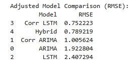
hybrid_pred = hybrid_forecast(df['productivity'])In the table below, I report the root mean squared error (RMSE) of each forecasting model. Because I’m only discussing model benchmarking, point forecast accuracy and run-time performance are the key metrics we’re interested in. And, because the data was generated without structural breaks and/or missing data, we’re only concerned about each model’s RMSE. I leave model uncertainty out of this discussion, and don’t compute confidence intervals (CIs). It’s important to keep in mind, however, that for inference applications the LSTM variants don’t natively support CIs due to their non-parametric nature. This can be overcome through resampling methods, such as bootstrapping and Monte Carlo Dropout.
The forecasting results are in line with the literature, in that they suggest:
- Regularization improves performance: corrected LSTM (with dropout/L2) outperforms base LSTM by 68.8% RMSE reduction (Sastry et al, 2025).
- Hybrid approach effectiveness: ARIMA-LSTM architectures leverage linear trend capture (ARIMA) and nonlinear residual modeling (LSTM), reducing errors in comparison to standalone models (Hamiane et al, 2024).
- Small-sample adaptations: Both ARIMA and LSTM corrections significantly outperform base versions.
Concluding remarks
The integration of new hire wage data into economic forecasting models presents a significant opportunity to enhance the accuracy and responsiveness of labor market analysis. Unlike average wages, new hire wages are markedly more procyclical, providing a sharper, real-time indicator of labor market turning points and productivity fluctuations. This responsiveness allows policymakers to better anticipate economic shifts and implement timely interventions, as new hire wages more accurately reflect marginal labor costs and adjust rapidly to evolving economic conditions. By capturing these dynamics, forecasts become more attuned to short-term cycles and can support more effective fiscal planning.
Equally promising is the adoption of advanced machine learning techniques, such as LSTM networks and hybrid ARIMA-LSTM models, which have demonstrated substantial improvements in forecasting accuracy - especially in the context of non-linear, volatile, or small-sample macroeconomic data. These methods can uncover complex temporal patterns and adapt to structural changes that traditional models may miss, further strengthening the empirical foundation of economic projections. The pace of methodological innovation in both theory and applied econometrics is accelerating, making it a great era for economic forecasters and policymakers alike. Staying abreast of these advancements is not only exciting but essential for ensuring that policy decisions are grounded in the best available evidence.