I have been spending the last two months creating econometrics and data science tasks to train AI models for OpenAI. The work is very interesting and a wonderful opportunity to dive deeper into certain methods and areas in the literature that I haven’t had as much opportunity to explore during my PhD. I have been especially interested in the intersection between traditional econometrics and machine learning, and what that intersection means for causal inference.

In one of my recent tasks I decided to try replicating a specific empirical demonstration from a paper I had read before but never sat down to fully reconstruct: Mullainathan and Spiess, Machine Learning: An Applied Econometric Approach, Journal of Economic Perspectives, 2017. One of their central insights is how regularisation techniques such as L1 (LASSO) are very useful to predict yhat in high-dimensional problems where the true DGP is sparse, but are not as useful for causal inference because LASSO will not always remove the same predictors in the same dataset, across partitions – that is, there is a dichotomy between predictor stability versus coefficient stability when using L1-regularisation. After simulating some data and trying to replicate the results, I used Claude to help me produce a visualisation that provides a satisfying geometric interpretation of what is happening in the hyperparameter space, and why this dichotomy is structural to l1-regularisation. This post is my attempt to explain it properly, with the geometry made visible.

1. Two Different Statistical Objectives

The paper’s opening argument is simple enough that it is easy to underestimate. Mullainathan and Spiess draw a distinction between two fundamentally different statistical objectives:

Predicting ŷ: minimising out-of-sample prediction error.
Estimating β: recovering the causal or structural relationship between a predictor and an outcome.

These are not just different goals. They lead to different estimators, different diagnostics, and, importantly, different notions of what stability means. Machine learning algorithms, LASSO included, are optimised for the first objective. They are not built for the second. This matters when one tries to use them for causal inference.

The paper’s Figure 2 is the empirical demonstration. Take a cross-sectional dataset of workers with log wages and 30+ predictors. Split the data into 10 random partitions. Fit LASSO on each partition with a fixed regularisation parameter. Record which variables get selected. Then ask: how stable is the selection across partitions, compared to how stable is out-of-sample R²?

The answer is interesting. Out-of-sample R² barely moves. The selection matrix is almost unrecognisable from one partition to the next.

Here is what that looks like when you build it in Stata.

2. The Selection Heatmap

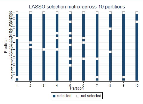
LASSO selection matrix across 10 partitions

Each row is a predictor (x1–x30). Each column is one of the 10 training partitions. A filled cell means LASSO assigned a nonzero coefficient to that predictor on that partition. An empty cell means it zeroed it out.

The heatmap is, I think, an intuitive illustration of this property. The selected variables shift substantially across columns. Some predictors appear in eight or nine partitions; others appear in two or three, or not at all. The pattern looks almost random in the sparse region of the heatmap.

Now look at the OOS metrics for those same ten runs, reported below from Stata’s tabstat after fitting and evaluating LASSO on each training/held-out split:

* OOS predictive metrics across 10 partitions
tabstat oos_r2 oos_rmse, statistics(mean sd min max) columns(statistics)

           |      mean        sd       min       max
-----------+-----------------------------------------
    oos_r2 |     0.3619     0.0325   0.3132    0.4099
  oos_rmse |     0.3558     0.0119   0.3352    0.3753

OOS RMSE — the scale-interpretable error in log-wage units — has a coefficient of variation of roughly 8% across partitions. The model predicts with essentially the same absolute accuracy everywhere. OOS R² is more variable, but that is almost entirely because the held-out outcome variance fluctuates across 50-observation partitions, not because predictive performance is genuinely unstable. The prediction surface is stable. The selection surface is not.

This is the result Mullainathan and Spiess wanted us to see. Predictive stability and coefficient stability are different objects.

3. Why Does This Happen? The L1 Geometry

To understand why this happens structurally, it is very useful to look at what LASSO is actually doing in the hyperparameter space. While the analytical formulation is, in my opinion, fairly intuitive, the geometric interpretation of what the equations tell us is particularly helpful and satisfying.

LASSO solves the following constrained problem:

\[\min_\beta \|y - X\beta\|_2^2 \quad \text{subject to} \quad \|\beta\|_1 \leq t\]

Think of the feasible region — the set of all β satisfying the L1 constraint — as a shape in coefficient space. In two dimensions it is a diamond. In three dimensions it is an octahedron. In 30 dimensions it is a hyperdiamond with 2³⁰ corners.

Now think of the loss function. The OLS solution is the unconstrained minimum. Around it, the loss surface forms concentric ellipsoids — level sets of equal prediction error. As we expand outward from the OLS solution, the first time one of these ellipsoids touches the L1 constraint region is the LASSO solution.

The key geometric fact: the L1 ball has corners and edges, and smooth ellipsoids hitting a spiky shape almost always make contact at a corner. At a corner, at least one coordinate is exactly zero. That is why LASSO produces exact zeros — and why Ridge, whose constraint region is a smooth sphere, almost never does.

I encourage you to test different calibrations in the interactive graph below. I used Claude to help me produce it in Javascript. Drag to rotate in 3D, scroll to zoom, and use the sliders to move the OLS solution and adjust λ.

The white sphere is the OLS solution β*. Concentric shells expand outward as loss ellipsoids. The blue octahedron is the L1 constraint ball. The gold wireframe ellipsoid is the first to touch the ball — its contact point is the green LASSO solution β̂.

You can also try the “near tipping point” preset: nudge β₁* and β₂* past each other using the sliders. Watch the green LASSO solution jump between two corners of the octahedron. The ellipsoid barely changes shape — prediction loss is nearly identical — but the contact point flips entirely. A completely different predictor is selected.

This is exactly what the heatmap was showing statistically. When the OLS solution sits roughly equidistant from two corners of the L1 ball, a tiny change in the training data — different observations in the partition — tips the tangency from one corner to the other. Different predictor selected. Same prediction ellipsoid. Same OOS R².

4. The Irrepresentable Condition: When Is Selection Actually Reliable?

There is a formal result that makes this precise. The irrepresentable condition (Zhao and Yu, 2006) states that LASSO will consistently recover the true support — the correct set of nonzero predictors — if and only if:

\[\|X_{S^c}'X_S(X_S'X_S)^{-1}\operatorname{sign}(\beta_S^*)\|_\infty < 1\]

where S is the true support and S^c is its complement. In plain language: no excluded predictor can be too correlated with the included ones, in the direction of the true coefficients.

When two predictors are highly correlated — say x1 and x2 with ρ = 0.85 in the synthetic dataset used here — the irrepresentable condition fails. The L1 penalty cannot afford to include both, so it is forced to pick one. But because both are nearly substitutable in terms of prediction loss, the choice is determined by noise-level fluctuations in the training data. x1 wins on one partition; x2 wins on another. The loss is nearly identical either way. The selected support is completely different.

We can verify this directly in Stata. After fitting the ten LASSO models, run correlate x1-x30. The high-correlation pairs — (x1, x2), (x7, x8), (x14, x15) — never appear selected simultaneously in the same partition across all ten runs. The geometry forbids it.

The selection frequency distribution below makes the instability quantitative:

* Selection frequency: fraction of 10 partitions in which each predictor is selected
tabstat sel_freq, by(predictor) statistics(mean) nototal

predictor |  sel_freq
----------+----------
       11 |    100%
       27 |    100%
        3 |    100%
       ...
       21 |     80%
        2 |     70%
       10 |     70%
       19 |     60%
       30 |     0%

Predictors with sel_freq closest to 100% correspond to the variables with the largest true coefficients in the data-generating process. The instability concentrates among weak-signal and collinear predictors.

The picture that emerges: a handful of predictors are robustly selected across partitions. Most are not. And OOS RMSE, the scale-interpretable error metric, barely moves regardless of which set of predictors was chosen.

5. Why This Matters for Causal Inference

Here is where the practical stakes become clear, and where I think the ML community sometimes underestimates the problem.

In prediction tasks, none of this matters. If your goal is to minimise RMSE on held-out data, coefficient instability is irrelevant. The ellipsoid level is what you care about, not which corner it touches. LASSO is excellent at this and produces genuinely stable predictions.

The problem arises when you use LASSO as a pre-screening step for causal inference. This is a common and superficially reasonable workflow: use LASSO to select variables from a high-dimensional set of controls, then run a structural causal model — a DiD, an IV regression, an event study — on the selected subset. The logic is appealing. Why not let a principled penalised regression tell you which covariates to include?

The answer is that the selected subset is a function of which corner the L1 ball tangency fell on, which is partly a function of which observations happened to be in your training sample. You are feeding sampling noise into your covariate selection, and that noise propagates directly into your causal estimate.

More concretely:

If the true confounders include x1 and x2, but x1 and x2 are correlated and LASSO only selects x1 on this partition, you have omitted a confounder. Your treatment effect estimate is biased.
If you had run the same analysis on a different random sample, LASSO might have selected x2 instead. Your causal estimate would be different, not because the data-generating process changed, but because the L1 geometry tipped the other way.
The OOS R² would look nearly identical in both cases. The prediction metrics give you no warning that the causal model has changed.

This is what the paper means when it says that ML algorithms are built for ŷ, not for β. The stability guarantee that ML tools provide — good generalisation, stable out-of-sample performance — is valuable. It just does not extend to the question of which variables matter causally.

6. Practical Implications

Let me close with four concrete takeaways, particularly for practitioners coming from an ML background.

1. Never use raw LASSO selection as input to a causal model without stability checking. At minimum, refit LASSO across multiple random splits and keep only predictors selected consistently — say, in at least 70–80% of runs.

2. Double selection (Belloni, Chernozhukov and Hansen, 2014) is the right tool when you need LASSO for high-dimensional covariate control in a causal setting. It runs LASSO on both the outcome and the treatment variable, takes the union of selected predictors, and then runs OLS on that union. The union step provides partial insurance against the instability.

3. The selection frequency distribution is a diagnostic, not a curiosity. A predictor selected in 9 of 10 partitions is genuinely informative. A predictor selected in 2 of 10 is a coin flip. Reporting selection frequencies alongside coefficient estimates should be standard practice whenever LASSO is used in a research context.

4. The instability is not a bug you can fix by tuning λ more carefully. It is a structural property of the L1 objective. As the dataset grows, LASSO converges to the correct support only if the irrepresentable condition holds — which is precisely the condition that fails when predictors are correlated, which is almost always.

The Mullainathan and Spiess paper is worth reading in full. But the empirical demonstration in Figure 2, which I reconstructed here in Stata, is the part that has stayed with me. I have always found it easier to understand difficult technical concepts when I can give them some sort of geometric interpretation and visualise what that function is doing to that input, be it a random variable, a function, some vector space or other objects. And this was one of those situations where it was, for me, especially helpful.

References

Mullainathan, S. and Spiess, J. (2017). Machine Learning: An Applied Econometric Approach. Journal of Economic Perspectives, 31(2), 87–106.

Zhao, P. and Yu, B. (2006). On Model Selection Consistency of Lasso. Journal of Machine Learning Research, 7, 2541–2563.

Belloni, A., Chernozhukov, V. and Hansen, C. (2014). High-Dimensional Methods and Inference on Structural and Treatment Effects. Journal of Economic Perspectives, 28(2), 29–50.

Hawinkel, S., Waegeman, W. and Maere, S. (2023). The Out-of-Sample R²: Estimation and Inference. arXiv:2302.05131.